BSc: Introduction to Optimization.F22

Introduction to Optimization

• Course name: Introduction to Optimization
• Code discipline: CSE???
• Subject area: Data Science and Artificial Intelligence

Short Description

The course outlines the classification and mathematical foundations of optimization methods, and presents algorithms for solving linear and nonlinear optimization. The purpose of the course is to introduce students to methods of linear and convex optimization and their application in solving problems of linear, network, integer, and nonlinear optimization. Course starts with linear programming and moving on to more complex problems. primal and dual simplex methods, network flow algorithms, branch and bound, interior point methods, Newton and quasi-Newton methods, and heuristic methods. Current states, literature, techniques, theories, and methodologies are presented and discussed during the semester.

Prerequisites

Prerequisite subjects

• CSE201: Mathematical Analysis I
• CSE202: Analytical Geometry and Linear Algebra I
• CSE203: Mathematical Analysis II
• CSE204: Analytical Geometry and Linear Algebra II

Prerequisite topics

• Basic programming skills.
• OOP, and software design.

Course Topics

Course Sections and Topics

Section	Topics within the section
Linear programming	Optimization Applications Formulation of Optimization Models Graphical Solution of Linear Programs Simplex Method Linear Programming Duality and Sensitivity Analysis
Nonlinear programming	Nonlinear Optimization Theory Steepest Descent and Conjugate Gradient Methods Newton and Quasi-Newton Methods Quadratic Programming
Extensions	Network Models Dynamic Programming Multi-objective Programming Optimization Heuristics

Intended Learning Outcomes (ILOs)

What is the main purpose of this course?

The main purpose of this course is to enable a student to go from an idea to implementation of different optimization algorithms to solve problems in different fields of studies like machine and deep learning, etc.

ILOs defined at three levels

We specify the intended learning outcomes at three levels: conceptual knowledge, practical skills, and comprehensive skills.

Level 1: What concepts should a student know/remember/explain?

By the end of the course, the students should be able to ...

• remember the different classifications and mathematical foundations of optimization methods
• remember basic properties of the corresponding mathematical objects
• remember the fundamental concepts, laws, and methods of linear and convex optimization
• distinguish between different types of optimization methods

Level 2: What basic practical skills should a student be able to perform?

By the end of the course, the students should be able to ...

• Funderstand the basic concepts of optimization problems
• evaluate the correctness of problem statements
• explain which algorithm is suitable for solving problems
• evaluate the correctness of results

Level 3: What complex comprehensive skills should a student be able to apply in real-life scenarios?

By the end of the course, the students should be able to ...

• understand the basic foundations behind optimization problems.
• classify optimization problems.
• choose a proper algorithm to solve optimization problems.
• validate algorithms that students choose to solve optimization problems.

Grading

Course grading range

Grade	Range	Description of performance
A. Excellent	90-100	-
B. Good	75-89	-
C. Satisfactory	60-74	-
D. Fail	0-59	-

Course activities and grading breakdown

Activity Type	Percentage of the overall course grade
Midterm	30
2 Intermediate tests	30 (15 for each)
Final exam	40

Recommendations for students on how to succeed in the course

• Participation is important. Attending lectures is the key to success in this course.
• Review lecture materials before classes to do well.
• Reading the recommended literature is optional, and will give you a deeper understanding of the material.

Resources, literature and reference materials

Open access resources

• Convex Optimization – Boyd and Vandenberghe. Cambridge University Press.

Closed access resources

• Engineering Optimization: Theory and Practice, by Singiresu S. Rao, John Wiley and Sons.
• Bertsimas, Dimitris, and John Tsitsiklis. Introduction to Linear Optimization. Belmont, MA: Athena Scientific, 1997. ISBN: 9781886529199.

Software and tools used within the course

• MATLAB
• Python
• Excel

Activities and Teaching Methods

Teaching and Learning Methods within each section

Teaching Techniques	Section 1	Section 2	Section 3
Problem-based learning (students learn by solving open-ended problems without a strictly-defined solution)	0	0	0
Project-based learning (students work on a project)	1	1	1
Modular learning (facilitated self-study)	0	0	0
Differentiated learning (provide tasks and activities at several levels of difficulty to fit students needs and level)	1	1	1
Contextual learning (activities and tasks are connected to the real world to make it easier for students to relate to them)	0	0	0
Business game (learn by playing a game that incorporates the principles of the material covered within the course)	0	0	0
Inquiry-based learning	0	0	0
Just-in-time teaching	0	0	0
Process oriented guided inquiry learning (POGIL)	0	0	0
Studio-based learning	0	0	0
Universal design for learning	0	0	0
Task-based learning	0	0	0

Activities within each section

Learning Activities	Section 1	Section 2	Section 3
Lectures	1	1	1
Interactive Lectures	1	1	1
Lab exercises	1	1	1
Experiments	0	0	0
Modeling	0	0	0
Cases studies	0	0	0
Development of individual parts of software product code	0	0	0
Individual Projects	1	1	1
Group projects	0	0	0
Flipped classroom	0	0	0
Quizzes (written or computer based)	0	0	0
Peer Review	0	0	0
Discussions	1	1	1
Presentations by students	1	1	1
Written reports	0	0	0
Simulations and role-plays	0	0	0
Essays	0	0	0
Oral Reports	0	0	0

Formative Assessment and Course Activities

Ongoing performance assessment

Section 1

1. A steel company must decide how to allocate next week’s time on a rolling mill, which is a machine that takes unfinished slabs of steel as input and can produce either of two semi-finished products: bands and coils. The mill’s two products come off the rolling line at different rates:

   Bands 200 tons/hr

   Coils 140 tons/hr.

   They also produce different profits:

   Bands $ 25/ton

   Coils $ 30/ton.

   Based on currently booked orders, the following upper bounds are placed on the amount of each product to produce:

   Bands 6000 tons

   Coils 4000 tons.

   Given that there are 40 hours of production time available this week, the problem is to decide how many tons of bands and how many tons of coils should be produced to yield the greatest profit. Formulate this problem as a linear programming problem. Can you solve this problem by inspection?

2. Solve the following linear programming problems.

   maximize $6x_{1}+8x_{2}+5x_{3}+9x_{4}$

   subject to $2x_{1}+x_{2}+x_{3}+3x_{4}\leq 5$

   $x_{1}+3x_{2}+x_{3}+2x_{4}\leq 3$

   $x1,x2,x3,x4\geq 0$

3. Give an example showing that the variable that becomes basic in one iteration of the simplex method can become nonbasic in the next iteration.
4. Solve the given linear program using the dual–primal two phase algorithm.

   maximize $2x_{1}-6x_{2}$

   subject to $-x_{1}-x_{2}-x_{3}\leq -2$

   $2x_{1}-x_{2}+x_{3}\leq 1$

   $x1,x2,x3\geq 0$

Section 2

1. Find the minimum of the function $f=\lambda /log\lambda$ using the following methods:
   • Newton method
   • Quasi-Newton method
   • Quadratic interpolation method
2. State possible convergence criteria that can be used in direct search methods.
3. Why is the steepest descent method not efficient in practice, although the directions used are the best directions?
4. What is the difference between quadratic and cubic interpolation methods?
5. Why is refitting necessary in interpolation methods?
6. What is a direct root method?
7. What is the basis of the interval halving method?
8. What is the difference between Newton and quasi-Newton methods?

Section 3

1. Solve the following LP problem by dynamic programming:

   Maximize $f(x_{1},x_{2})=10x_{1}+8x_{2}$

   subject to $2x_{1}+x_{2}\leq 25$

   $3x_{1}+2x_{2}\leq 45$

   $x_{2}\leq 10$

   $x1,x2\geq 0$

   Verify your solution by solving it graphically.

2. Consider the following tree solution for a minimum cost network flow problem:

   

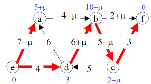
   As usual, bold arcs represent arcs on the spanning tree, numbers next to the bold arcs are primal flows, numbers next to non-bold arcs are dual slacks, and numbers next to nodes are dual variables.

   • For what values of is this tree solution optimal?
   • What are the entering and leaving arcs?
   • After one pivot, what is the new tree solution?
   • For what values of is the new tree solution optimal?

Final assessment

Section 1

1. Solve the following linear programming problems.

   maximize $x_{1}+3x_{2}$

   subject to $-x_{1}-x_{2}\leq -3$

   $-x_{1}+x_{2}\leq -1$

   $-x_{1}+2x_{2}\leq 2$

   $x1,x2\geq 0$

2. Give an example showing that the variable that becomes basic in one iteration of the simplex method can become nonbasic in the next iteration.
3. Solve the given linear program using the dual–primal two phase algorithm.

   maximize $6x_{1}+8x_{2}+5x_{3}+9x_{4}$

   subject to $x_{1}+x_{2}+x_{3}+x_{4}=1$

   $x_{1},x_{2},x_{3},x_{4}\geq 0$

Section 2

1. Perform two iterations of the steepest descent method to minimize the function given from the stated starting point $(-1.2,1)$

   $f(x_{1},x_{2})=100(x_{2}-x_{1}^{2})^{2}+(1-x_{1})^{2}$

2. Minimize $f=2x_{1}^{2}+x_{2}^{2}$ by using the steepest descent method with the starting point $(1,2)$ (two iterations only).
3. Minimize $f=x_{1}^{2}+3x_{2}^{2}+6x_{3}^{2}$ by Newton's method using the starting point as $(2,-1,1)$ .

Section 3

• It is proposed to build thermal stations at three different sites. The total budget available is 3 units (1 unit = $10 million) and the feasible levels of investment on any thermal station are 0, 1, 2, or 3 units. The electric power obtainable (return function) for different investments is given below. Find the investment policy for maximizing the total electric power generated.

Return function Ri(x)	i = 1	i = 2	i = 3
R0(x)	0	0	0
R1(x)	2	1	3
R2(x)	4	5	5
R3(x)	6	6	6

• A fertilizer company needs to supply 50 tons of fertilizer at the end of the first month, 70 tons at the end of the second month, and 90 tons at the end of the third month. The cost of producing x tons of fertilizer in any month is given by $$(4500x+20x^{2})$. It can produce more fertilizer in any month and supply it in the next month. However, there is an inventory carrying cost of $400 per ton per month. Find the optimal level of production in each of the three periods and the total cost involved by solving it as an initial value problem.
• Consider the following tree solution for a minimum cost network flow problem:

  

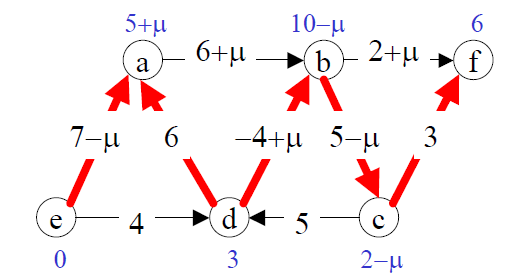
  As usual, bold arcs represent arcs on the spanning tree, numbers next to the bold arcs are primal flows, numbers next to non-bold arcs are dual slacks, and numbers next to nodes are dual variables.

  For what values of is this tree solution optimal?

  What are the entering and leaving arcs?

  After one pivot, what is the new tree solution?

  For what values of is the new tree solution optimal?

The retake exam

Retakes will be run as a comprehensive exam, where the student will be assessed the acquired knowledge coming from the textbooks, the lectures, the labs, and the additional required reading material, as supplied by the instructor. During such comprehensive oral/written the student could be asked to solve exercises and to explain theoretical and practical aspects of the course.